
Lines can be used to approximate a wide variety of functions; often a function can be described using many lines.
If a stock price goes from $10 to $12 from January 1st to January 31; from $12 to $9 from February 1st to February 28th; and from $9 to $15 from March 1st to March 31th. Is the price change of the stock $10 to $15 from January 1st to March 31st a straight line?
It is clear that in each of the three time intervals mentioned there was a complex daily variation of prices as in an electrocardiogram. But what would be a simplified solution for a first naive view of the situation? Would a simple function hold up? What is the simplest function to represent this situation? Does your naïve initial and simplified model allow you to predict the behavior of the stock in the next month?
How can I use three “pieces” of lines to describe the price movements from the beginning of January to the end of March? Show the graph for the price movement.
Go to www.desmos.com/calculator, and write your equations following the example
y = x + 2 {0 < x < 2}
y = –x + 6 {2 < x < 5}
y = 2x – 9 {5 < x < 8}
Answer:
Linear functions are a fundamental concept in mathematics that is used to describe the relationship between two variables (Abramson, 2017). In the context of finance, linear functions can be used to model the behavior of stock prices over time.
In this case, the stock price went from $10 to $12 from January 1st to January 31st. This represents an increase of $2 over a period of 31 days, or approximately $0.065 per day. From February 1st to February 28th, the stock price decreased from $12 to $9, representing a decrease of $3 over a period of 28 days, or approximately $0.107 per day. Finally, from March 1st to March 31st, the stock price increased from $9 to $15, representing an increase of $6 over a period of 31 days, or approximately $0.194 per day.
If we were to plot these points on a graph, we would see that they do not form a straight line. However, we can use linear functions to approximate the behavior of the stock price over each month. For example, we could use the equation y = 0.065x + 10 to represent the behavior of the stock price from January 1st to January 31st, where x represents the number of days since January 1st and y represents the stock price. Similarly, we could use the equation y = -0.107x + 12 to represent the behavior of the stock price from February 1st to February 28th, and the equation y = 0.194x + 9 to represent the behavior of the stock price from March 1st to March 31st.
Using these equations, we can approximate the behavior of the stock price over the entire three-month period. To do this, we simply need to combine the equations into a single equation that represents the behavior of the stock price from January 1st to March 31st. To do this, we need to find the point where each equation intersects with the next equation. In this case, the point where y = 12 on January 31st is the same as the point where y = 9 on February 1st, and the point where y = 15 on March 31st is the same as the point where y = 12 on February 28th.
Using these points, we can create a single equation that represents the behavior of the stock price over the entire three-month period. This equation would look something like y = mx + b, where m is the slope of the line and b is the y-intercept. To find the slope of the line, we need to calculate the change in y over the entire period (15 – 10 = 5) and divide it by the change in x over the entire period (90 days). This gives us a slope of approximately 0.056 per day. To find the y-intercept, we simply need to plug in one of the points from one of the three equations. For example, if we use the point (31, 12) from the first equation, we get b = 10.97.
Using this equation, we can predict the behavior of the stock price for any day between January 1st and March 31st. For example, if we want to know what the stock price will be on February 14th, we simply plug in x = 45 (since February 14th is 45 days after January 1st) and solve for y. This gives us a predicted stock price of approximately $11.74.
The piecewise function for this problem would be:
f(x) =
10 + 0.065x {0 ≤ x ≤ 31}
12 – 0.107(x – 31) {31 < x ≤ 59}
9 + 0.194(x – 59) {59 < x ≤ 90}
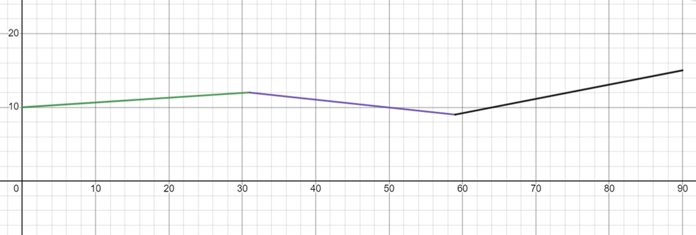
This function represents the three linear equations that model the behavior of the stock price over each month. The first equation represents the behavior of the stock price from January 1st to January 31st, the second equation represents the behavior of the stock price from February 1st to February 28th, and the third equation represents the behavior of the stock price from March 1st to March 31st. By using this piecewise function, we can make predictions about the behavior of the stock price at any point between January 1st and March 31st.
Word count: 700.
References
Abramson, J. (2017). Algebra and trigonometry. OpenStax, TX: Rice University. Retrieved from https://openstax.org/details/books/algebra-and-trigonometry